How much labelling should you include in a visualisation?

The inspiration for this post, and for the visualisation(s) accompanying it, comes from two places. One, from my last post, where I considered the importance of white space – when considering every text element, does it really need to be there? The other inspiration was from the latest work from Nicholas Rougeux below:

The original is on Nicholas’ webpage http://www.c82.net. Now I love the text-free look, and the patterns that emerge from the data. From the context of the title, and its presentation within the website, I know this is a visual timeline relating to the elements of the periodic table, and the patterns emerge from the fact that order of discovery and atomic number don’t follow the same timeline, until the most recent heaviest artificially-created elements.

However, look closely, and you’ll see the text very lightly included – date of discovery and name of every element is in small text in slightly lighter purple. This completes the visualisation perfectly – you don’t need to see this text to appreciate the art, but you can examine the text to analyse the meaning of each curve.

I found some data (well, typed in some stuff from Wikipedia into Excel – same thing), loaded it up and started to explore some visualisations.

A few days ago, I posted the following tweet:

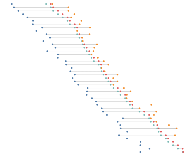
How easy is it to recognise a dataset and the story it is telling us? Here’s an unlabelled first viz looking at a dataset: My question is (for a future blog post): can any of you recognise what this is depicting without the help of any labels whatsoever? pic.twitter.com/nm4bwEcfzI

— Neil Richards (@theneilrichards) January 17, 2018

… with this accompanying image

Before I continue and give clues as to what this refers to – it’s only fair to say I was corrected in the semantics of this tweet. And when it’s Storytelling with Data‘s own Cole Knaflic who corrects you, then you stand corrected! Cole correctly pointed out that it’s not the dataset that tells us the story, but we that tell the story with the data.

I’m going to pick on semantics here… I don’t think the data ever “tells a story.” People tell a story with the data. Maybe not your point, just wanted to raise. In any case, I have no idea what this data is, so curious what this may turn into!

— Cole Knaflic (@storywithdata) January 17, 2018

I won’t argue with those semantics (though I do wonder if it’s as simple as that, but there are plenty of other posts where storytelling is discussed at length). Cole was right – it wasn’t my point, but I was delighted the interest my post was generating!

As alluded to in the tweet, I removed all labels for marks, points, axes and titles, and wondered whether anyone could work out what the chart referred to. If you don’t want spoilers (and haven’t seen my original message and replies) then you might want to try it yourself.

I knew it wouldn’t be possible for everyone to work out. But it would be a fun exercise … and I genuinely thought some people might get this! It was hard for me to know how easy or otherwise it might be – since I knew the context. I knew the data I’d loaded up, I knew the labels I’d removed, and I knew the inspiration I had before setting the whole thing up (timelines, moving start points …)

I was really pleased with the response. Of course, my social media bubble is not the general public. It’s not people who are interested in the subject matter of the visualisation (and I haven’t even told you what that is yet!). It’s almost all enthusiasts and practitioners of data visualisation. A specialist audience – far more likely to solve the riddle than your average person. The result of this was a number of suggestions which intelligently considered things I hadn’t even considered myself. In approximate order:

• Jamie L spotted the relationship between the pairs of coloured dots, and that it represented 45 different things (could that be a clue?!), ordered by the red dot
• Andy Y submitted a series of emojis which I think indicated he was both intrigued and baffled. I’m rubbish at emojis though, he could have been scared and hungry for all I know, sorry Andy!
• Louis A thought it would be related to political party polling, since the colours would fit well
• Mark E wondered on the significance of the colours, and whether it was intentional that a few near the bottom are unconnected (yes!)
• Mike C knew that they had to be events connected by time but was unsure of the order – does the fact that the unconnected lines with no yellow dot are all at the bottom mean that most recent are on top?
• Mark E was then convinced it must be related to DNA/chromosomes since there were 46 observations (this is unlucky – a lot of sense to this guess but there are actually 45!)
• Mike C thought it looked like positions in a race, with each of the four dots always in the same sequence, but why was one team/competitor so far in the lead?!
• Ian R then got very close … “Time on the horizontal. Blue is birth, yellow death. Green becoming something, red ceasing to be that something. British PMs? Poet Laureate?”
• Sophie W was the first to get it spot on, with one word: “Presidents”. And well done also to Vince B who got it later, independently.

So, combine Ian and Sophie’s answers and you have it exactly right. Here’s what it might have looked like labelled: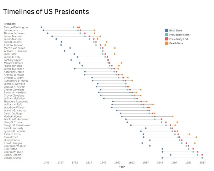

Here’s a sensibly labelled version. Now we get it – Lincoln, Roosevelt, Kennedy (and more) who died in office. Carter, Clinton and Trump among those still alive. A legend to show what each of those pesky coloured dots mean.

Now of course it wasn’t possible to get this from the original (though well done to those that did). I had the context – the timeline inspiration, the fact that I knew the dataset, but I gave nothing to those who saw the unlabelled version. Without knowing this, making the most intelligent leaps can make you jump to conclusions in the wrong direction:

• Looks like 46 groups of four – is it do to with chromosomes/DNA?
• I think it looks like a timeline but there’s incomplete data – is most recent on top?
• I don’t know what dataset Neil has here but he often visualises sport when practicing – is it sport data? Neil is British, are these Prime Ministers?
• These colours look significant – are they sport teams or political parties?

The clues to the fact that these are presidents are there, but only if you *know* they are there! 45 entries – most without a fourth (death) entry at the end; some unexplained entries where the red dot is closer than usual to the teal dot and the yellow dot is hidden behind it (those presidents who died in office). But the key is that the user needs to have enough information in the first place to then enjoy exploring and finding these anomalies in the visualisation, not have to go in reverse and work out the visualisation meaning by spotting the pattern quirks (though admittedly it’s a fun challenge for some!)

Sophie gave me some additional context too which shows that it certainly wasn’t instantly gettable without the combined wisdom of the crowd – she didn’t get it straight away and thought that it might be related to gender pay gaps. Only after seeing some of the guesses evolve and seeing Jamie’s initial observation that there were 45 lines did the penny drop. She also asked “What do I win?” Nothing I’m afraid – but I did promise I’d publicise her excellent data journalism related newsletter “Fair Warning” – subscribe to it here! https://tinyletter.com/FairWarning/

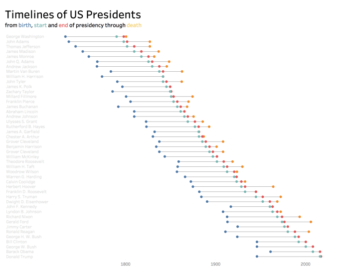
So, for those who are still reading – what might it look like? My own preference is to avoid legends unless they’re crucial, or interactive. By drawing the legend colour into the explanatory text away from the graph, we reclaim some white space. If we have to have y-axis labels (and yes, I admit, of course we do), we don’t need the heading that says “President”. Perhaps we can fade their text colour? Similarly we don’t need to tell the reader that those numbers in the 1700s to 2000s are years, I think (s)he can work that out. I’ll leave in the years but have far fewer points.

It’s not perfect but it’ll do and it’s an interesting visualisation to bring up this particular debate question. Is it my final visualisation? Well, no. You don’t take inspiration from a Nicholas Rougeux art piece to start your next work and not come up with something a little more fun. I’d love to publish this post with my finalised visualisation in place but at the moment it’s still a work in progress.

I’m interested in the way the blue dots are asynchronous – the dates of birth of presidents are far from the order of their inaugurations (in much the same way that chemical elements are not discovered in weight order). So what does the timeline look if we order all events: birth, death, inauguration and end of presidency, along the same timeline?

The result is fascinating but you’ll see why this is a work in progress – one of the most interesting takeaways is what makes it so difficult to visualise! Presidents 42,43 and 45 (Clinton, Bush, Trump) are all born within a couple of months of each other, hence their timelines cluster together. This is best seen on a very wide resolution – click on the link below for full wide version (sorry phone readers), and even then you’ll see how close they are together. In choosing to label the numbers rather than the president names (which is not uncommon in the US) it emphasises some of these anomalies (the youth of Obama compared to Trump, for example).

I also like the way it shows how 20th and 21st century Presidents are much more likely to live into their nineties but I’d love to find a way of showing the number of past and present living Presidents at any one time.

I think I’ve got two options from here – either to build in a bit more interactivity (such as the president details/biogs on hover so as to clarify this), or to go for something a little different. The blog started with abstract curves on timelines – I wasn’t sure that was the way to go with this. But it’s an interesting dataset and I’m open to possibilities – feedback and ideas for V2 and beyond are welcome!